Section 1 Introduction
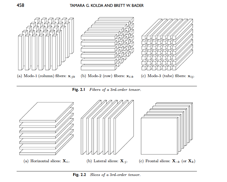
A tensor is a multidimensional array, where the order of tensor denotes the dimension of the array. For example, a scalar is simply an order-0 tensor, a vector order-1, a matrix order-2, and any tensor with order-3 or greater is described as a higher order tensor. For this paper I will be focusing on the simplest higher-order tensor, the order-3 tensor, which can be visualized as a sort of Rubik's cube.
Section 2 3rd-Order Tensor Decompositions
Subsection 2.1 Modal Operations
To discuss the Higher Order SVD, we must first have a general understanding of two modal operations, modal unfoldings and modal products.
Definition 2.1 Modal Unfolding
Suppose \(\mathcal{A}\) is a 3rd-order tensor and \(\mathcal{A} \in \mathbb{R}^{n_1 \times n_2 \times n_3}\). Then the modal unfolding \(\mathcal{A}_{(k)}\) is the matrix \(\mathcal{A}_{(k)} \in \mathbb{R}^{n_k \times N}\) where \(N\) is the product of the two dimensions unequal to \(n_k\).
Definition 2.2 Modal Product
The modal product, denoted \(\times_{k}\), of a 3rd-order tensor \(\mathcal{A} \in \mathbb{R}^{n_1 \times n_2 \times n_3}\) and a matrix \(\textbf{U} \in \mathbb{R}^{J \times n_k}\), where \(J\) is any integer, is the product of modal unfolding \(\mathcal{A}_{(k)}\) with \(\textbf{U}\). Such that
\[\textbf{B}=\textbf{U} \mathcal{A}_{(k)} = \mathcal{A} \times_{k} \textbf{U}\]
Subsection 2.2 Higher Order SVD (HOSVD)
Informally the Higher Order SVD is simply defined as an SVD for each of the tensors modal unfoldings.
Definition 2.3 Higher Order SVD
Suppose \(\mathcal{A}\) is a 3rd-order tensor and \(\mathcal{A} \in \mathbb{R}^{n_1 \times n_2 \times n_3}\). Then there exists a Higher Order SVD such that
\[\textbf{U}^{T}_{k}\mathcal{A}_{(k)}=\Sigma_{k} \textbf{V}^{T}_{k} \quad (1\leq k \leq d)\\\]
where \(\textbf{U}_{k}\) and \(\textbf{V}_{k}\) are unitary matrices and the matrix \(\Sigma_{k}\) contains the singular values of \(\mathcal{A}_{(k)}\) on the diagonal, \([\Sigma_{k}]_{ij}\) where \(i=j\), and is zero elsewhere.
Subsection 2.3 Rank of Higher Order Tensors
The notion of rank with respect to higher order tensors is not as simple as the rank of a matrix.
Definition 2.4 Rank of a Tensor
The rank of a tensor\(\mathcal{A}\) is the smallest number of rank 1 tensors that sum to \(\mathcal{A}\).
Subsection 2.4 CANDECOMP/PARAFAC Decomposition
Unfortunately there is no single algorithm to perform a CP decomposition on any tensor. This is partially due to the fact that the rank of a higher order tensor is not known precisely until a CP decomposition has been performed and is known to be the most concise decomposition.
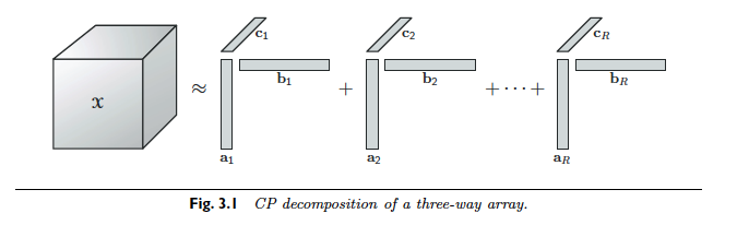
Definition 2.5 CP Decomposition
A CP decomposition of a 3rd-order tensor, \(\mathcal{A}\), is defined as a sum of vector outer products, denoted \(\circ\), that equal or approximately equal \(\mathcal{A}\). For \(R = rank(\mathcal{A})\)\[\mathcal{A} = \sum_{r=1}^{R}a_r \circ b_r \circ c_r\]
and for \(R \lt rank(\mathcal{A})\)\[\mathcal{A} \approx \sum_{r=1}^{R}a_r \circ b_r \circ c_r\]
Performing a CP decomposition on a 3rd order tensor \(\mathcal{A}\) is a matter of performing a Alternating Least Squares (ALS) routine to minimize \(||\mathcal{A}_{(1)} - \textbf{A}(\textbf{C}\odot \textbf{B})^T||\). To perform an ALS routine on this system, the system is divided into 3 standard least squares problems where 2 of the 3 matrices are held constant and the third is solved for. The main problem in implementing an ALS routine such as this, is choosing initial values for the two matrices that are held constant to initialize the first least squares problem. This method may take many iterations to converge, the point of convergence is heavily reliant on the initial guess, and the computed solution is not always accurate. Faber, Bro, and Hopke (2003) investigated six methods as an alternative to the ALS method and none of them came out more effective than ALS in terms of accuracy of solution, but some did converge faster [6]. In addition, derivative methods have been developed that are superior to the ALS method in terms of convergence and solution accuracy but are much more computationally expensive [3]. For quantum mechanical problems involving a few \(3 \times 3 \times 3\) tensors accuracy is paramount to computational expense. One such algorithm is the PMF3 algorithm described in Paatero (1997) which computes changes to all three matrices simultaneously. This allows for faster convergence than the ALS method and optional specificity for non-negative solutions reduces divergence in systems that are known to have positive solutions [5].
Section 3 Application to Quantum Chemistry
Subsection 3.1 Introduction of the Problem
In the field of quantum chemistry, linear algebra is heavily utilized and higher order tensors can arise in some specialized problems. In my personal experience, I have encountered 3rd-order tensors while working with the spectroscopic properties of molecules. In practice the issues arise when trying to manipulate 3rd-order tensors, and specifically when trying to rotate a 3rd-order tensor analogous to how a matrix would be rotated for a change in coordinates. For these problems the 3rd-order tensors can arise as an outer product between a matrix and a vector that represent the polarizability and dipole moment, respectively, of a molecule, the outer product of which is the hyperpolarizability tensor. In this case the method used to rotate the hyperpolarizability tensor is to rotate the vector and matrix independently and then recalculating the outer product after each rotation. This method maybe more computationally expensive and could result in numerical inaccuracies after repeated iterations, especially when dealing with small values. This solution is the only one that could be found by my colleagues and me. The true issue arises when the hyperpolarizability tensor is calculated independently by the computational program unless an intuitive user explicitly specifies the separate polarizability and dipole moments, but even then the outer product of the polarizability and dipole moment is only approximately equal to the hyperpolarizability tensor. For this reason it is desirable to have a way to rotate the hyperpolarizability tensor independently.
Subsection 3.2 Rotation Matrices
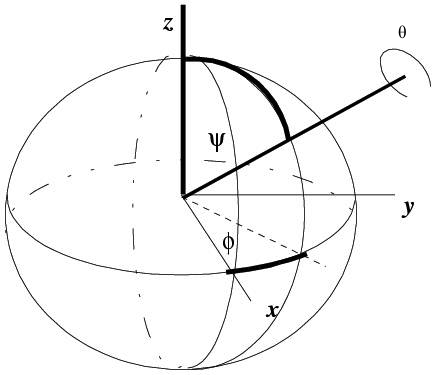
In the context of linear algebra and quantum chemistry, a rotation matrix is a matrix that is used to rotate a set of points in space. In the specific context of spectroscopy, a rotation matrix is used to rotate a molecules properties, such as hyperpolarizability represented by a 3rd-order tensor, about an axis or axes. This process is done to orientationally average molecules over axes that are known to allow free rotation. The rotation matrix commonly used to do this is below and the corresponding axes of rotation are shown in Figure 1 [2], \[R = \begin{bmatrix} \cos (\phi ) \cos (\psi )-\cos (\theta ) \sin (\phi ) \sin (\psi ) & -\cos (\theta ) \cos (\psi ) \sin (\phi )-\cos (\phi ) \sin (\psi ) & \sin (\theta) \sin (\phi ) \\ \cos (\psi ) \sin (\phi )+\cos (\theta ) \cos (\phi ) \sin (\psi ) & \cos (\theta ) \cos (\phi ) \cos (\psi )-\sin (\phi ) \sin (\psi ) & -\cos (\phi ) \sin (\theta ) \\ \sin (\theta ) \sin (\psi ) & \cos (\psi ) \sin (\theta ) & \cos (\theta ) \\ \end{bmatrix}\] It is immediately evident that the rotation matrix gets complex quickly when rotating an object in 3 dimensions around 3 rotational axes. Despite the complexity, this matrix still maintains a very nice property that all rotational matrices have in common, they are unitary. This is significant because it gives us an easy-to-find inverse for an otherwise complex looking matrix and determinant \(1\) guarantees the matrix operated on by the rotation matrix will not be stretched or compressed.
Subsection 3.3 Rotation by CP Decomposition
The most natural solution to this problem after reviewing the decompositions of higher order tensors is to use a CP decomposition. Above it is shown that the CP decomposition produces a sum of vectors, so to rotate a 3rd order tensor we can simply rotate each of the vectors individually by the same angle and then perform the necessary outer products and summations to form the rotated 3rd order tensor. This is mathematically illustrated for the case of \(\mathcal{X} \in \mathbb{R}^{3 \times 3 \times 3}\) where there exists a CP decomposition. In this particular problem we also know that using a value of \(r=3\) will provide an exact decomposition because the tensor should be the outer product of a \( 3 \times 3\) matrix and vector in \(\mathbb{R}^3\) so the resulting tensor should have the same rank as the matrix. Since the matrix is a calculated numerical matrix, its rank is almost certainly 3, thus the tensor rank is 3. Fortunately in this situation, unlike most, the tensor rank is unambiguous so we can write, \[\mathcal{X} = \sum_{j=1}^{3}a_j \circ b_j \circ c_j\] . Then, \begin{align} \mathcal{X}_{Rot} & = \sum_{j=1}^{3} (R a_j) \circ (R b_j) \circ (R c_j)\notag\\ & = [R a_1|R a_2|R a_3] \odot [R b_1|R b_2|R b_3] \odot [R c_1|R c_2|R c_3]\notag\\ & = R[a_1|a_2|a_3] \odot R[b_1|b_2|b_3] \odot R[c_1|c_2|c_3]\notag\\ & = R\textbf{A} \odot R\textbf{B} \odot R\textbf{C}\notag\\ & = [[R\textbf{A},R\textbf{B},R\textbf{C}]]\notag \end{align} This results in only an additional 3 matrix multiplications, which are computationally cheap, but the CP decomposition is computationally expensive. In this case where our 3rd-order tensor is relatively small, the more accurate but more computationally intense PMF3 algorithm can be utilized over the ALS method. This is very beneficial because often in these computations every decimal point is significant and sometimes the number are very small making it more difficult to distinguish between a numerical zero and a significant number. Another thing to keep in mind is that this procedure only applies to a \(3 \times 3 \times 3\) system or a \(2 \times 2 \times 2\) (with a \(2\times 2\) rotational matrix) because rotational matrices have no larger analogs, so the tensors will always be relatively small. However, the decomposition is still nontrivial and is not guaranteed to converge in every situation.
Subsection 3.4 Proposal of a 3rd-Order Rotational Tensor
Disclaimer: This portion is not necessarily mathematically accurate and will be rather conversational.
After spending hours searching, I have been unable to come across a higher order tensor analog to a rotational matrix. In the literature they repeatedly refer to rotating a 3rd-order tensor as, \[\mathcal{X}^{\prime}_{ijk}=R_{li}R_{mj}R_{nk}\mathcal{X}_{lmn}\] but have never been able to find the matrices that behave in this manner plus I would expect that the 3rd-order tensor would have to be rotated by another 3rd-order tensor. For this reason I have been trying to figure out a way to construct a rotational tensor. While working with the CP decomposition and rotation by multiplying each of the vectors with a rotational matrix, I thought what if I did a similar routine multiplying different combinations of the standard unit vectors with a rotational matrix to form the entries of a 3rd-order rotational tensor. \[\mathcal{R}=\sum R e_i \circ R e_j \circ R e_k\] It is often said it is good enough to see what a matrix/linear transformation does on a basis, so if the right basis was used this could be used to form a 3rd-order rotational tensor. In addition, after such a tensor is created, it would be difficult to define it as a rotational tensor because it is hard to translate the concepts like unitary, inverse, and determinant into terms of a higher order tensor.